3 ways to run tutorials in OpenFOAM
Tutorials - The starting point of almost every simulation
Tutorials are an interactive way of transferring knowledge. They are a kind of recipe that provides you with the necessary steps to complete a particular task. The maintainers of OpenFOAM deliver an extensive collection of tutorials together with the library. For OpenFOAM users, the supplied case setups are the most useful information provided for free. Reading this post to the end will enable you to run all these tutorials, avoiding some pitfalls.
Tutorials are essential because to start your project in most cases you will:
- Select a solver implementing all necessary physics
- Check the available tutorials for the solver
- Copy, rename, and modify the most similar tutorial
- Test and run your simulation
The tutorial collection contains a variety of different case setups. In the following, you will learn three different ways to run OpenFOAM tutorials. To get started, open a terminal window and copy the tutorial collection into your run directory.
cp -r $FOAM_TUTORIALS $FOAM_RUN
1. Simple blockMesh/mySolverFoam tutorials
The lid-driven cavity flow is a common test case for validation. It is also one of the cases thoroughly explained in the OpenFOAM tutorial guide (section 2.1). The way how you create and run simulations in OpenFOAM may seem a bit strange to users who come from a Microsoft-Windows environment or who are used to have a GUI. Instead, solvers, utilities, or scripts in OpenFOAM require a certain directory structure containing control files. Navigate to the cavity folder and type ls -R or tree to get an overview.
cd $FOAM_RUN/tutorials/incompressible/icoFoam/cavity/
tree
.
├── 0
│   ├── p
│   └── U
├── constant
│   └── transportProperties
└── system
    ├── blockMeshDict
    ├── controlDict
    ├── fvSchemes
    └── fvSolution
All tutorials have a system (control files for solvers and utilities), a constant (mesh, material properties), and a 0 (zero; technically, the initial time folder could have any value/name but 0 is the most common scenario) directory (initial values, boundary conditions). If no further execution scripts are provided, you will always have to run blockMesh, for the mesh creation, and afterward your solver of choice, in our case icoFoam. In rare cases, there are one or two more dictionaries for preprocessing in the system folder (pre - they are executed before the solver). A possible scenario is an additional setFieldsDict to set initial field values. The corresponding utility to run after blockMesh would be setFields. The applications will give some output which should be saved in log files for later use (and to avoid that the terminal window is overflowing with solver output). &> redirects the standard output and error messages of, for example, blockMesh to the file log.blockMesh. Now it’s time to run our first tutorial:
blockMesh &> log.blockMesh
# ... maybe some more preprocessing utilities
icoFoam &> log.icoFoam
 |
|---|
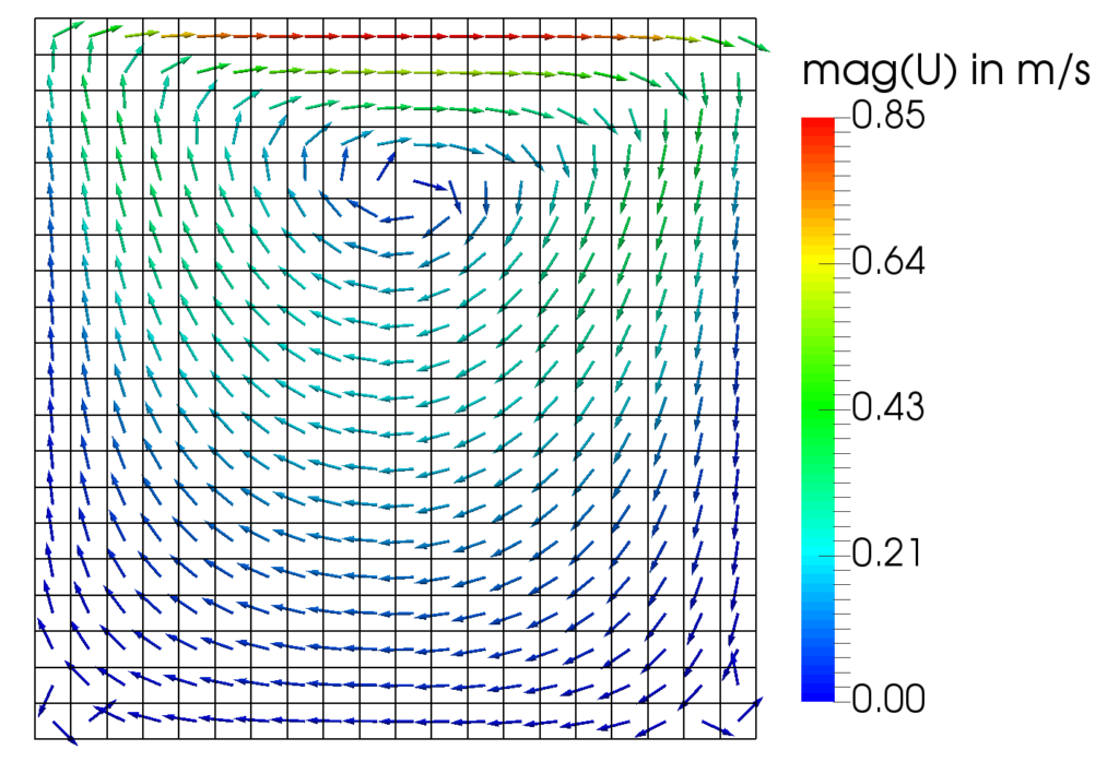
| Vector plot of cell-centered velocity colored by its magnitude. |
2. Tutorials with Allrun/Allclean scripts
The reactingParcelFilmFoam solver is, as one can guess from the name, a fairly complex application involving many physical models. Pre- and post-processing tasks for such simulations are correspondingly extensive. At this point, running every single application with its options would be too time (and nerve) consuming. Luckily, automating processes comes naturally within a Linux environment via Shell scripts. Basically, all necessary commands are written into a file which is then executed. In the tutorial collection, these scripts are usually called Allrun. For convenience, different scripts can be created for subtasks, e.q. meshing or parallel execution. After the setup is complete, you may want to run a variety of simulations with different parameters. Here it comes in handy to have an Allclean script, which resets the case to its initial state. All of this you can find in the hotBoxes tutorial.
cd $FOAM_RUN/tutorials/lagrangian/reactingParcelFilmFoam/hotBoxes
tree -L 1
.
├── 0.org
├── Allclean
├── Allrun
├── Allrun-parallel
├── Allrun.pre
├── constant
...
└── system
Running the tutorial in serial takes about 24h. So it’s wise to run it overnight or/and to use the Allrun-parallel script, which runs the solver with four processes in parallel (about 9h to complete on my office laptop).
./Allrun
 |
|---|
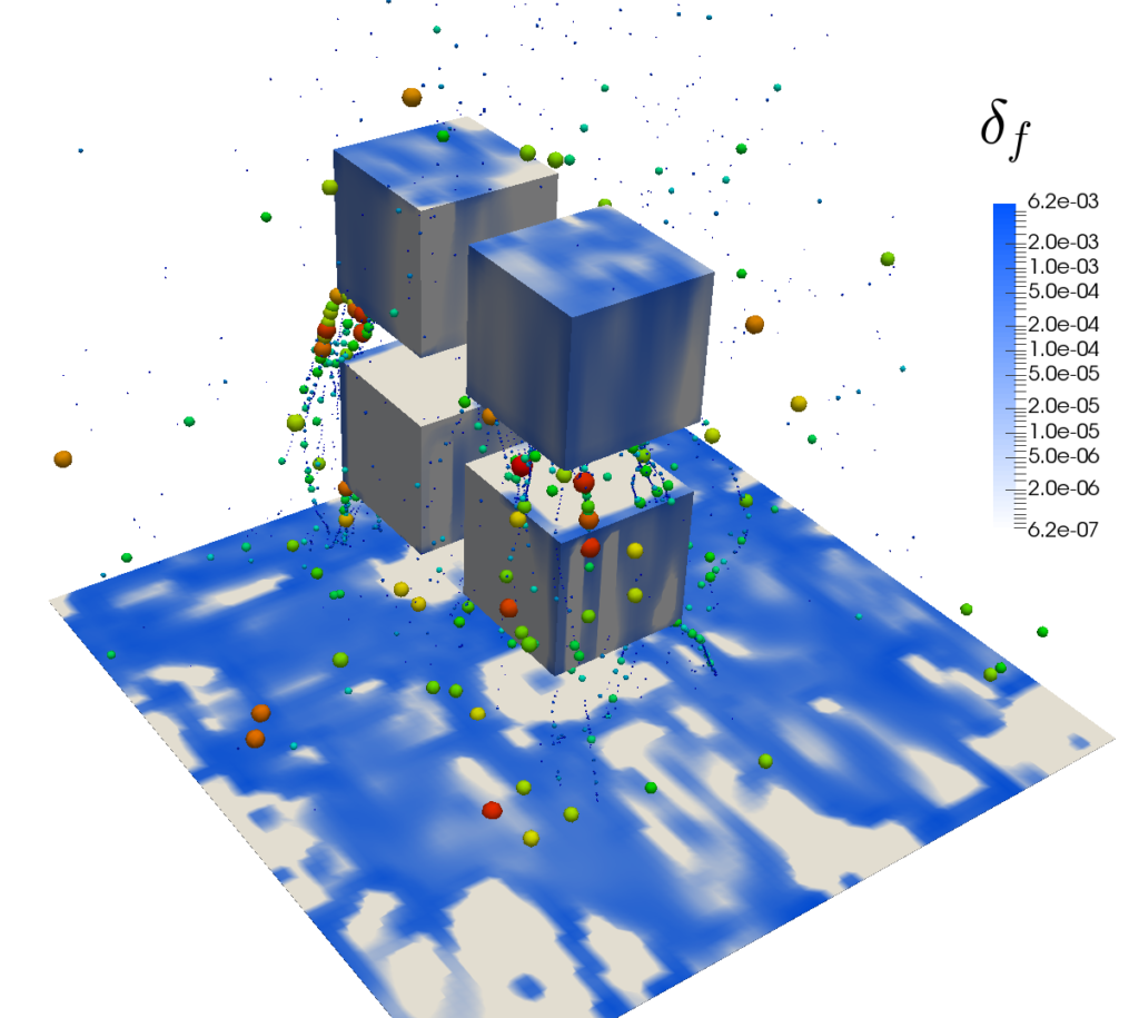
| The surface color indicates the thickness of the cooling film. The Lagrangian particles’ diameters scale with the mass they carry. |
3. Tutorials that require system operations
The last type of tutorials I want to introduce here need system operations. System operations basically means that an application (e.g., a solver) compiles and (hopefully) runs user-supplied C++ source code at runtime. Examples are the #codeStream directive or the codedFixedValue boundary condition (same link as before). Since the OpenFOAM 2.3.1 release, system calls are allowed by default. If you run an older version or you want to check your configuration, open the system-wide controlDict and set the allowSystemOperations switch to 1.
# for a system-wide installation root privileges are required
# e.g on Ubuntu run
sudo gedit $FOAM_ETC/controlDict
// and set the allowSystemOperations switch to 1
InfoSwitches
{
...
    // Allow case-supplied C++ code (#codeStream, codedFixedValue)
    allowSystemOperations   1;
}
Now we are ready to simulate the potential flow around a cylinder. This case is very charming because it allows us to validate our numerical results with an analytical solution. Within the case’s controlDict a coded function object is supplied which later on calculates the numerical error as defined in the picture below. So let’s run the simulation!
cd $FOAM_RUN/tutorials/basic/potentialFoam/cylinder
blockMesh &>log.blockMesh
potentialFoam &>log.potentialFoam
Here is a task for you:
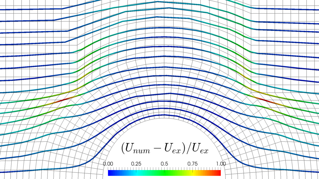
- Take a close look at the streamlines in the picture below. First, check the alignment between mesh and streamlines. Can you spot under which conditions the highest deviations occur?
- Open the fvSolution file located in the system directory, set different values for the nNonOrthogonalCorrectors (0, 1, 2, …), and re-run the simulation. How does the error behave?
 |
|---|
| The color of the streamlines indicates the relative difference between numerical and analytical solution. |
That’s it for this tutorial! With the above information, you are prepared to explore all the tutorials coming with OpenFOAM.
Cheers, Andre